Popular data processing platforms offer users the ability to inject an external process into the data processing pipeline. The data flowing through the data pipeline is fed as input to the external process, while the output produced by the process is fed back into the pipeline. The external process runs an executable or a script. This pattern resembles the popular Unix pipelines (or pipes). This feature is usually found under the name of Streaming.

In Apache Hadoop, streaming is achieved with the Hadoop Streaming utility. In Apache Spark, streaming is achieved with the RDD.pipe function. (Not to be confused with Spark Streaming which is used for a different purpose.)

SciDB provides this ability through the stream plug-in. Besides the usual pattern of injecting an external process into the data pipeline, the SciDB plug-in offers user-friendly and efficient interfaces for the Python and R languages. Specifically:

The external process can be a Python or R script;
The code for the external process does not have to be available on the SciDB server a priori, instead, it can be sent from the client;
The input and output data can be in the form of Pandas DataFrames in Python and R DataFrames in R. Internally the data is transferred using Apache Arrow for Python and native format for R.

The following diagram provides the intuition of how streaming works in SciDB. Notice the green octagons marked with R. They represent the external processes injected into the data pipeline. Data gets transferred to and from them using stdin and stdout respectively. There are as many instances of the external process as there are SciDB instances.

SciDB Streaming

In this post, we explore a few useful patterns of interacting with the SciDB Stream plug-in from Python. As an example, we use the Python scikit-learn machine-learning library and build a model for the Digit Recognizer data-science competition offered by Kaggle. The dataset used in this competition is the Modified National Institute of Standards and Technology (MNIST) handwritten image dataset.

Setting Up

First, we need to install the stream plug-in for SciDB. Installation instructions are available as part of the plug-in README.md file. The Apache Arrow library is also installed at this point. We also use the accelerated_io_tools plug-in for loading the data into SciDB. See here for the installation instructions. (The accelerated_io_tools plug-in was discussed in more detail in an earlier post.) Finally, we install the limit plug-in for its ability limiting the output results. A Docker image file of SciDB and all these plug-ins is available here.

Since our entire solution is in Python we need to install a number of Python packages. Some are only necessary on the machines which run SciDB (server side) while others are only necessary on the machine from which we connect to SciDB (client side):

SciDB-Py: Python interface to SciDB (only necessary on the client side);
SciDBStrm: Python helper package for the SciDB stream plug-in (necessary on both client and server side);
scikit-learn: Machine learning in Python package (only necessary on the server side);
SciPy: Fundamental library for scientific computing in Python (only necessary on the server side).

The NumPy and Pandas packages are also installed as dependencies. All of these packages can be installed using pip:

# Client side
pip install scidb-py sklearn scipy dill feather-format pandas
pip install git+http://github.com/paradigm4/stream.git@python#subdirectory=py_pkg

# Server side
pip install dill feather-format pandas
pip install git+http://github.com/paradigm4/stream.git@python#subdirectory=py_pkg

Next, we need to download the train and test datasets offered by Kaggle as part of the Digit Recognizer data-science competition. Downloading the datasets might require creating an account on the Kaggle website. The datasets need to be copied onto SciDB instance 0.

Preparing the Training Data

We start by loading and preprocessing the training data. We load the train.csv data file using the aio_input operator from the accelerated_io_tools plug-in. In the CSV file, each record contains a label for the image and the pixel color intensity of each pixel in the image. The data format is described in detail on the competition data page. We want to load the label in one SciDB attribute and all the pixels in a second SciDB attribute. So, we use the aio_input operator to separate the label in one attribute and leave the rest in the error field of the operator output. We will parse the error field in the next step. The AFL query looks like this:

# iquery --afl --no-fetch
AFL% store(
       aio_input(
         'path=/kaggle/train.csv',
         'num_attributes=1',
         'attribute_delimiter=,',
         'header=1'),
       train_csv);
Query was executed successfully

The query assumes the Kaggle training data file, train.csv, is in the /kaggle directory on the first SciDB server instance (instance 0). We can have a look at the resulting array using the limit operator:

# iquery --afl
AFL% limit(train_csv, 3);
{tuple_no,dst_instance_id,src_instance_id} a0,error
{0,0,0} '1','long,0,0,0,...'
{1,0,0} '0','long,0,0,0,...'
{2,0,0} '1','long,0,0,0,...'

As intended, the first attribute a0 contains the record label (0, 1, 2, etc.) while the error attribute contains the pixel color intensities (e.g., 0,0,0,..., etc.).

Next, we convert the pixel color intensities values from text to binary. This is the first use of the stream plug-in. We implement this step entirely in Python, using the SciDB-Py library (see docs). The code for this step is:

import scidbpy
import scidbstrm

def map_to_bin(df):
    import numpy

    df['a0'] = df['a0'].map(int)
    df['error'] = df['error'].map(
        lambda x: numpy.array(map(int, x.split(',')[1:]),
                              dtype=numpy.uint8).tobytes())
    return df

db = scidbpy.connect()
ar_fun = db.input(upload_data=scidbstrm.pack_func(map_to_bin)).store()

que = db.stream(
    db.arrays.train_csv,
    scidbstrm.python_map,
    "'format=feather'",
    "'types=int64,binary'",
    "'names=label,img'",
    '_sg({}, 0)'.format(ar_fun.name)
).store(
    db.arrays.train_bin)

The code has three parts:

Declare the mapping function map_to_bin;
Upload the code of the mapping function to a temporary array in SciDB;
Use the stream operator to apply the mapping function to each record in the train_csv array. Store the result in the train_bin array.

The mapping function takes as input a DataFrame with a chunk of records from the train_csv array. The function uses the pandas.Series.map function, which applies a map function to a DataFrame column. It first converts the label value, in the a0 column, from string to integer. It then converts the pixel color intensities, in the error column, from string to binary. The lambda function provided parses the pixel color intensities and stores the result into a NumPy array. The binary representation of the NumPy array is stored back into the DataFrame. The mapping function is serialized using the pack_func function provided by the SciDBStrm library (see docs) and uploaded to a temporary array in SciDB. This array will be removed by the SciDB-Py library when the Python interpreter exits.

In the stream operator, the mapping function is provided using the _sg operator. This operator can pass a second array as an argument to the stream operator. The 0 argument in the _sg operator instructs SciDB to copy the array to every instance. The script to be executed by the stream operator is provided in the second argument, and, in this case, it is set to scidbstrm.python_map. With this argument, a standard Python invocation is used (see docs). The code loads the mapping function provided in the second array argument and applies it to the first array argument. The output array attribute types and names are provided as part of the stream arguments as well. In this case, the output attribute types are int64 and binary. The resulting array looks like this:

# iquery --afl
AFL% limit(train_bin, 3);
{instance_id,chunk_no,value_no} label,img
{0,0,0} 1,<binary>
{0,0,1} 0,<binary>
{0,0,2} 1,<binary>

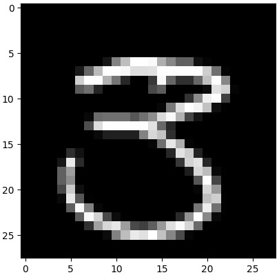
Each record stores the image label as integer and the pixel color intensities as the binary representation of a NumPy. The image of a record can be displayed in IPython using:

%matplotlib gtk  # replace gtk with a back-end available for your platform
import matplotlib.pyplot

plt = matplotlib.pyplot.imshow(
          numpy.frombuffer(
              db.limit(db.arrays.train_bin, 1)[0]['img']['val'],
              dtype=numpy.uint8).reshape((28, 28)),
         cmap='gray')

Matplotlib screenshot

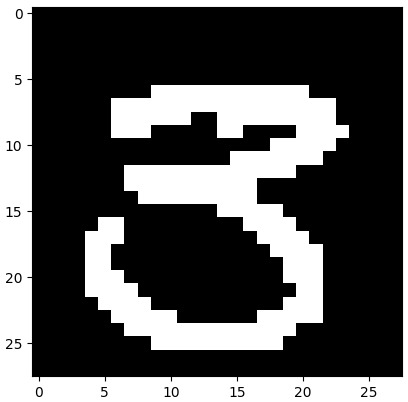
Finally, we are going to convert the training data images from grayscale to black and white. We do this with the help of the stream operator using a similar pattern as before:

def map_to_bw(df):
    import numpy

    def bin_to_bw(img):
        img_ar = numpy.frombuffer(img, dtype=numpy.uint8).copy()
        img_ar[img_ar > 1] = 1
        return img_ar.tobytes()

    df['img'] = df['img'].map(bin_to_bw)
    return df

que = db.iquery("""
store(
  stream(
    train_bin,
    {script},
    'format=feather',
    'types=int64,binary',
    'names=label,img',
    _sg(
      input(
        {{sch}},
        '{{fn}}',
        0,
        '{{fmt}}'),
      0)),
  train_bw)""".format(script=scidbstrm.python_map),
                upload_data=scidbstrm.pack_func(map_to_bw))

As before, the stream mapping function leverages the pandas.Series.map function. The function provided to pandas.Series.map converts the binary value stored in the img column to a NumPy array and applies the black and white thresholding. The binary representation of the modified NumPy array is stored back into the DataFrame.

For calling the stream operator, we are making use of the iquery function. This pattern allows us more flexibility, but it is not as user-friendly as the db.stream approach. Moreover, we avoid creating a temporary array for the mapping function by combining the input operator with the _sg operator. Avoiding to create the temporary array could result in performance benefits. The resulting array is very similar to the one before:

# iquery --afl
AFL% limit(train_bw, 3);
{instance_id,chunk_no,value_no} label,img
{0,0,0} 1,<binary>
{0,0,1} 0,<binary>
{0,0,2} 1,<binary>

The image of a record can be displayed in IPython as before:

plt = matplotlib.pyplot.imshow(
          numpy.frombuffer(
              db.limit(db.arrays.train_bw, 1)[0]['img']['val'],
              dtype=numpy.uint8).reshape((28, 28)),
         cmap='gray')

Matplotlib screenshot

Training a Model

We now train a model on the data we just uploaded. We train the model in SciDB using the stream plug-in. Since SciDB is a distributed database, we first train multiple models in parallel on each SciDB instance and then we merge all the models into a single global model. For the instance models, we use the stochastic gradient descent classifier available in the scikit-learn library. One reason we choose this model is its ability to train on partial data. This is useful as the data is streamed one chunk at a time and not available all at once. So, we invoke the classifier’s partial_fit (see docs) function for each chunk. The Python code for training the instance models is:

class Train:
    model = None
    count = 0

    @staticmethod
    def map(df):
        img = df['img'].map(
            lambda x: numpy.frombuffer(x, dtype=numpy.uint8))
        Train.model.partial_fit(numpy.matrix(img.tolist()),
                                df['label'],
                                range(10))
        Train.count += len(df)
        return None

    @staticmethod
    def finalize():
        if Train.count == 0:
            return None
        buf = io.BytesIO()
        sklearn.externals.joblib.dump(Train.model, buf)
        return pandas.DataFrame({
            'count': [Train.count],
            'model': [buf.getvalue()]})


ar_fun = db.input(upload_data=scidbstrm.pack_func(Train)).store()

python_run = """'python -uc "
import io
import numpy
import pandas
import scidbstrm
import sklearn.externals
import sklearn.linear_model

Train = scidbstrm.read_func()
Train.model = sklearn.linear_model.SGDClassifier()
scidbstrm.map(Train.map, Train.finalize)
"'"""

que = db.stream(
    db.arrays.train_bin,
    python_run,
    "'format=feather'",
    "'types=int64,binary'",
    "'names=count,model'",
    '_sg({}, 0)'.format(ar_fun.name)
).store(
    db.arrays.model)

The code structure is similar as before, except that instead of a mapping function, we provide a “mapping” class. We do this for two reasons:

We want to provide both a map and a finalize function. The map function is called for each chunk. The finalize function is called once all the chunks have been processed.
We want to have two static class variables to keep track of the model and a count of how many training records were used. (This could have been global variables in the script we provide to stream, but it is more intuitive to have them as class variables.)

The map function uses the pandas.Series.map function to convert the values in the img column from binary to NumPy. We then use the NumPy array (reshaped as a matrix) and the label column to train a partial model. We also keep track of how many records we used to train. The map function does not return any data back to SciDB.

The finalize function first checks whether any training data was fed into the model. Remember that this code runs independently on each SciDB instance and some instances might have no training data. If training data was provided, the model is serialized using the dump function (see docs) and returned to SciDB along with the training records count.

For this step, we provide a customized Python script to the stream operator. The script is stored in the python_run variable and it invokes the Python interpreter the Python code for this step as a command-line argument. After importing the required modules, we deserialize the Train class (provided to the stream operator as the second argument using the _sg operator) using the scidbstrm.read_func function (see docs). We then initialize our model and apply the map and finalize functions on the streamed data using the scidbstrm.map function (see docs). The resulting array looks is like this:

# iquery --afl
AFL% scan(model);
{instance_id,chunk_no,value_no} count,model
{0,0,0} 22949,<binary>
{1,0,0} 19051,<binary>

Our setup consists of two SciDB instances and each had approximately 50% of the training data. As a result, two models have been trained in parallel, one on each instance.

Next, we merge the instance models in a single global model. For the global model, we choose the voting classifier for its ability to combine multiple trained models. The Python code for this step is:

def merge_models(df):
    import io
    import pandas
    import sklearn.ensemble
    import sklearn.externals

    estimators = [sklearn.externals.joblib.load(io.BytesIO(byt))
                  for byt in df['model']]
    if not estimators:
        return None

    labelencoder = sklearn.preprocessing.LabelEncoder()
    labelencoder.fit(range(10))

    model = sklearn.ensemble.VotingClassifier(())
    model.estimators_ = estimators
    model.le_ = labelencoder

    buf = io.BytesIO()
    sklearn.externals.joblib.dump(model, buf)

    return pandas.DataFrame({'count': df.sum()['count'],
                             'model': [buf.getvalue()]})


ar_fun = db.input(upload_data=scidbstrm.pack_func(merge_models)).store()

que = db.redimension(
    db.arrays.model,
    '<count:int64, model:binary> [i]'
).stream(
    scidbstrm.python_map,
    "'format=feather'",
    "'types=int64,binary'",
    "'names=count,model'",
    '_sg({}, 0)'.format(ar_fun.name)
).store(
db.arrays.model_final)

We use the standard pattern of providing a mapping function, called merge_models. In this function, we first deserialize the instance models. We also prepare a label encoder with 10 labels, one for each digit. Once we have this, we can instantiate the voting classifier and set its estimators and label encoder. The classifier is then serialized and returned to SciDB along with a total count of the training records.

Before calling the stream operator, we need to make sure that all the instance models are at one SciDB instance, in one chunk. This is done using the redimension operator (see docs). Getting all the instance models at one instance in one chunk does not present a scalability challenge since the number of models equals the number of SciDB instances. The resulting array contains one trained model and a training record count equal to the size of the training data:

# iquery --afl
AFL% scan(model_final);
{instance_id,chunk_no,value_no} count,model
{0,0,0} 42000,<binary>

Making Predictions

Now that we have a trained model, we are ready to make predictions on the test data. We start by loading the test data in SciDB:

# iquery --afl --no-fetch
AFL% store(
       input(
         <img:string>[ImageID=1:*],
         '/kaggle/test.csv',
         0,
         'csv:lt'),
       test_csv);
Query was executed successfully

The query assumes the Kaggle test data file, test.csv, is in the /kaggle directory on the first SciDB server instance (instance 0). We use the input operator (see docs) as opposed to the aio_input operator we used earlier because input assigns a sequential number (captured by ImageID) to each line of the input file. We need this because there are no explicit image IDs in the data file. Using t in the csv:lt format specifier, we instruct SciDB to look for TAB as the fild delimiter. Since our actual field delimiter is the comma, we force all the pixel color intensities into a single attribute, img. The resulting array looks like this:

# iquery --afl
AFL% limit(test_csv, 3);
{ImageID} img
{1} '0,0,0,...'
{2} '0,0,0,...'
{3} '0,0,0,...'

We use the stream operator and the model already stored in SciDB to make predictions. The Python code for this step is:

class Predict:
    model = None

    @staticmethod
    def csv_to_bw(csv):
        img_ar = numpy.array(map(int, csv.split(',')), dtype=numpy.uint8)
        img_ar[img_ar > 1] = 1
        return img_ar

    @staticmethod
    def map(df):
        img = df['img'].map(Predict.csv_to_bw)
        df['img'] = Predict.model.predict(numpy.matrix(img.tolist()))
        return df

ar_fun = db.input(
    upload_data=scidbstrm.pack_func(Predict)
).cross_join(
    db.arrays.model_final
).store()

python_run = """'python -uc "
import dill
import io
import numpy
import scidbstrm
import sklearn.externals

df = scidbstrm.read()
Predict = dill.loads(df.iloc[0, 0])
Predict.model = sklearn.externals.joblib.load(io.BytesIO(df.iloc[0, 2]))
scidbstrm.write()

scidbstrm.map(Predict.map)
"'"""

que = db.apply(
    db.arrays.test_csv,
    'ImageID',
    'ImageID'
).stream(
    python_run,
    "'format=feather'",
    "'types=int64,int64'",
    "'names=Label,ImageID'",
    '_sg({}, 0)'.format(ar_fun.name)
).store(
    db.arrays.predict_test)

We define a “mapping” class in order to have a static class variable for storing the trained model (instantiated during streaming). The class provides a transformation function (csv_to_bw) to convert a test record from text format to NumPy and to apply the black and white thresholding. (These transformations are identical with the one used for the training data earlier.) The actual map function first applies the transformation function for each record of the input DataFrame. Next, it predicts the labels for each of the images in the input DataFrame (after first reshaping the input DataFrame to a matrix). The labeled data is returned to SciDB.

In order to have both the “mapping” class we just defined and the model trained earlier available in the stream operator, we store both of them, as two attributes in a record in a temporary array. This temporary array is fed into the stream operator as the second argument array (using the _sg operator).

The Python script to be used by the stream operator is provided explicitly and stored in the python_run variable. The script starts by reading the first available chunk. The read function is part of the low-level SciDBStrm API which allows us to read chunks of data from SciDB (see docs). This first chunk is the chunk containing the second argument array we are providing using the _sg operator. From this chunk, we extract the “mapping” class and store it in Predict. The “mapping” class is the first attribute, of the first record, of the chunk, and we use iloc[0, 0] to extract it. We also extract the trained model and store it in Predict.model. The model is the third attribute, after the cross_join, and we use iloc[0, 2] to extract it. Since we are using the low-level streaming API we need to make an explicit call to write (this tells SciDB that we have no output for this first chunk of data). The script then proceeds by applying the Predict.map function to the streamed data. Once the stream operator is executed, the resulting array looks like this:

# iquery --afl
AFL% limit(predict_test, 3);
{instance_id,chunk_no,value_no} Label,ImageID
{0,0,0} 2,1
{0,0,1} 0,2
{0,0,2} 9,3

In our final step, we save the array containing the predictions on the client in a format consistent with the one expected by Kaggle. This can be done in Python using:

df = db.arrays.predict_test.fetch(as_dataframe=True)
df['ImageID'] = df['ImageID'].map(int)
df['Label'] = df['Label'].map(int)
df.to_csv('results.csv',
          header=True,
          index=False,
          columns=('ImageID', 'Label'))

The resulting file, results.csv, can be directly uploaded to Kaggle for scoring. We also made predictions for the training data. We plotted the true labels and the predicted labels on a scatter plot. We randomly jittered each point so that they do not completely overlap.

True vs. predicted labels

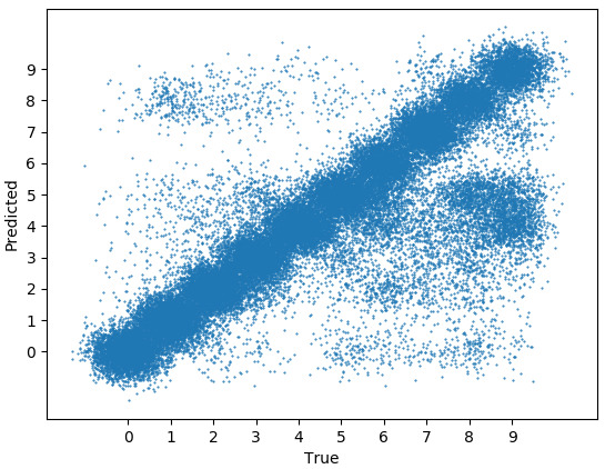
As we can see, most of the points are on the main diagonal, meaning that most of the data is labeled correctly. Moreover, there is a visible hot spot in the (9, 4) area, meaning that a lot of images of 9 are labeled as 4 by our model. The code for generating this plot is included in the full script

Summary

To summarize, in this post we looked at how we can use the stream operator to train machine-learning models in parallel in SciDB. As an example, we used the Python scikit-learn machine-learning library and trained a model for a data-science competition on Kaggle. The patterns we discussed were:

Use the stream operator with a mapping function;
Use the stream operator with a “mapping” class;
Provide a custom script to the stream operator;
Provide multiple values as second array arguments to the stream operator;
Store and retrieve NumPy arrays as binary values in SciDB;
Store and retrieve serialized machine-learning models in SciDB.

The code discussed here is available as a single script as part of the SciDBStrm Python package. A Docker image file of SciDB and required plug-ins for running this script is available here.

Machine Learning in SciDB

Leveraging the SciDB Stream plug-in